From Frustration to Fast: Using Ray for Parallel Computing on a Single Machine or a Cluster

If you're someone who works with data and runs computationally-intensive tasks, you know that multiprocessing can be a game changer. It can speed up your work significantly and save you precious time. I previously used the multiprocessing Python package for running my jobs concurrently, but that didn’t always go straightforward. I often had challenges when using multiprocessing in jupyter, and it also didn’t deal with errors well. Sometimes I experienced that the jobs would get stuck if the code raised an error without logging the error appropriately.

That's where Ray comes in. Ray is a Python library that has been a real lifesaver for me. It's not only lightning-fast and user-friendly, but it also allows you to distribute your tasks across multiple machines for even faster computation. Additionally, it offers built-in integrations for machine learning and data streaming.

While there are good resources available online for using Ray on a single machine (like this one), there's limited information on how to use it to distribute tasks across multiple machines and manually set up a cluster. As someone who has recently explored this feature of Ray, I want to share my experience with you in this blog post. If you're interested in speeding up your computations and making the most of Ray's capabilities, keep reading!

I'll first walk you through a simple simulation of SGD (stochastic gradient descent) and how to parallelize it for faster computation. We'll start by parallelizing the simulation on a single machine using Ray, and then we'll take things up a notch by distributing the task across multiple machines.

SGD on OLS

In this section, I'll provide some background on the simple SGD job that we'll be parallelizing using Ray. Let's consider the ordinary least squares (OLS) setting, where we have n observations of covariates x and independent variables y, and they have a linear relationship in the form of \(y = x^T \beta + \epsilon\), where \( \beta \) is the unknown vector of coefficients and epsilon is the error term. Our goal is to obtain an estimate of \( \beta \) using the SGD algorithm. Of course, you can simply use the OLS close-formed solution. :)

The SGD algorithm is an iterative optimization technique that randomly selects a data point and updates the estimates of the coefficients based on the error between the predicted and actual values. In each iteration, the algorithm updates the estimate of beta using the gradient of the loss function with respect to beta.

For this problem, our data-generating process looks like this

n = 10000
d = 100

X = np.random.normal(size=(n, d))
beta = np.random.normal(size=(d, 1))
eps = 0.1 * np.random.normal(size=(n, 1))
Y = X @ beta + eps

Where X is the pooled matrix with each row containing one of the covariate observations, and y is the stacked version of the independent variable.

The SGD method takes one of the data points at random and updates the estimate using the gradient of the estimation loss.

idx = np.random.randint(n)
x_step, y_step = X[idx, :].reshape(1, -1), Y[idx]
grad_step = gradient_step(x_step, y_step, beta_hat)
beta_hat -= lr * grad_step

The complete function looks like this, where I also store the series of step losses and a log of estimates and distances to the true parameter.

def gradient_step(x_step, y_step, beta_hat):
   return -x_step.T @ (y_step - x_step.dot(beta_hat))


def sgd_loss(X, Y, T, beta, lr=0.01):
   n, d = X.shape
   beta_hat = np.random.normal(size=(d, 1))
   loss_array = np.zeros(T)
   dist_array = np.zeros(T)
   estimate_log_every = 100
   estimate_array = np.zeros((T // estimate_log_every, d))
   for t in range(T):
       idx = np.random.randint(n)
       x_step, y_step = X[idx, :].reshape(1, -1), Y[idx]
       grad_step = gradient_step(x_step, y_step, beta_hat)
       beta_hat -= lr * grad_step
       step_loss = (y_step - x_step.dot(beta_hat)) ** 2
       loss_array[t] = step_loss[0, 0]
       dist_array[t] = np.linalg.norm(beta_hat - beta)
       if (t + 1) % estimate_log_every == 0:
           estimate_array[(t + 1) // estimate_log_every, :] = beta_hat.reshape(-1)
   return loss_array, dist_array, estimate_array

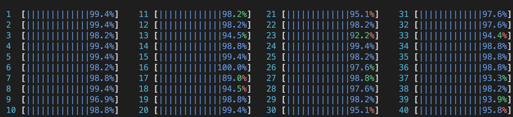
Running this function for T = 80000 and 100 repetitions without multiprocessing takes 3 min and 19s for me.

T = 80000
rounds = 100
estimate_log_every = 100


all_results_single = []
start_time = time.time()
for r in trange(rounds):
   result = sgd_loss(X, Y, T, beta=beta, lr=lr, estimate_log_every=estimate_log_every)
   all_results_single.append(result)
duration = time.time() - start_time
print(f"Runs using single process took {duration:.3f} seconds")

Multiprocessing on a Single Machine

The process starts with installing ray. You could simply do

pip install ray

or

pip install -U "ray[default]"

if you want to have the ray dashboard, a web application that shows how the runs are going, you can access the logs for each run.

Then you only need to do these steps

1. import ray

2. Add @ray.remote annotator to your function. Let's say the function has the name my_func

3. Call ray.init()

4. Run the function concurrently using ray.get([my_func.remote() for r in range(rounds)])

In my code, because I wanted both single-process and multiprocess versions of the function, I created a new function for the remote case that just calls the SGD function.

@ray.remote
def sgd_loss_remote(X, Y, T, beta, lr, estimate_log_every):
   return sgd_loss(X, Y, T, beta, lr, estimate_log_every)

Running the processes then looks like:

ray.init()
start_time = time.time()
all_results_remote = ray.get(
   [
       sgd_loss_remote.remote(
           X, Y, T, beta=beta, lr=lr, estimate_log_every=estimate_log_every
       )
       for r in range(rounds)
   ]
)
duration = time.time() - start_time
print(f"Runs using multiple processes took {duration:.3f} seconds")

This way, it only takes 16 seconds to finish! I got a significant win on time by using all of the CPU cores just after adding a few lines.

Run a ray cluster manually

Ray offers documentation for setting up Ray clusters on AWS or GCP servers, as well as utilizing Kubernetes. If these options align better with your requirements, I recommend referring to the documentation for detailed instructions. However, keep reading the post if you want to avoid the initial steps of setting up Kubernetes or wish to use Ray on your machines. In this section, I will focus on the scenario where you prefer to run a Ray cluster on multiple machines manually.

To start this, you need at least two machines in a network setting that can access each other. You also should ensure that both Python environments have ray and other packages required by your code. One of the machines will serve as the master (head), and other machines (workers) will connect to it.

First, you need to run ray on the head node using

​​ray start --head

You may face a question asking whether you want to share usage statistics that you can answer yes or no.

The response should look like this:

--------------------
Ray runtime started.
--------------------

Next steps
  To connect to this Ray runtime from another node, run
    ray start --address='192.168.1.2:6379'

  Alternatively, use the following Python code:
    import ray
    ray.init(address='auto')

  To connect to this Ray runtime from outside of the cluster, for example to
  connect to a remote cluster from your laptop directly, use the following
  Python code:
    import ray
    ray.init(address='ray://<head_node_ip_address>:10001')

  If connection fails, check your firewall settings and network configuration.

  To terminate the Ray runtime, run
    ray stop

As the output suggests, you now need to connect workers to the head using

ray start --address='{HEAD_NODE_IP}:6379'

Remember to change the IP address with the IP of the head node.

The response will be like:

--------------------
Ray runtime started.
--------------------
To terminate the Ray runtime, run
  ray stop

Now, to run your Python code, you need to do

ray job submit --address='{HEAD_NODE_IP}:6379' --working-dir . -- python main.py

The working dir line is critical, specifically if your code uses other local files and packages. The output would be like this:

Job submission server address: http://127.0.0.1:8265
2023-05-09 19:13:16,062 INFO dashboard_sdk.py:360 -- Package gcs://_ray_pkg_6c68afec082a1408.zip already exists, skipping upload.
-------------------------------------------------------
Job 'raysubmit_BAUvdD7m5EWcYXix' submitted successfully
-------------------------------------------------------
Next steps
  Query the logs of the job:
    ray job logs raysubmit_BAUvdD7m5EWcYXix
  Query the status of the job:
    ray job status raysubmit_BAUvdD7m5EWcYXix
  Request the job to be stopped:
    ray job stop raysubmit_BAUvdD7m5EWcYXix
Tailing logs until the job exits (disable with --no-wait):
2023-05-09 19:13:18,128 INFO worker.py:1230 -- Using address 10.155.105.194:6379 set in the environment variable RAY_ADDRESS
2023-05-09 19:13:18,128 INFO worker.py:1342 -- Connecting to existing Ray cluster at address: 192.168.1.2:6379...
2023-05-09 19:13:18,136 INFO worker.py:1519 -- Connected to Ray cluster. View the dashboard at 127.0.0.1:8265 
Runs using multiple processes took 9.233 seconds
------------------------------------------
Job 'raysubmit_BAUvdD7m5EWcYXix' succeeded
------------------------------------------

It now takes only 11 seconds, and I’m running on 76 CPU cores.

If you have installed the ray with the default option, you can see the dashboard at the head ip address on port 8265.

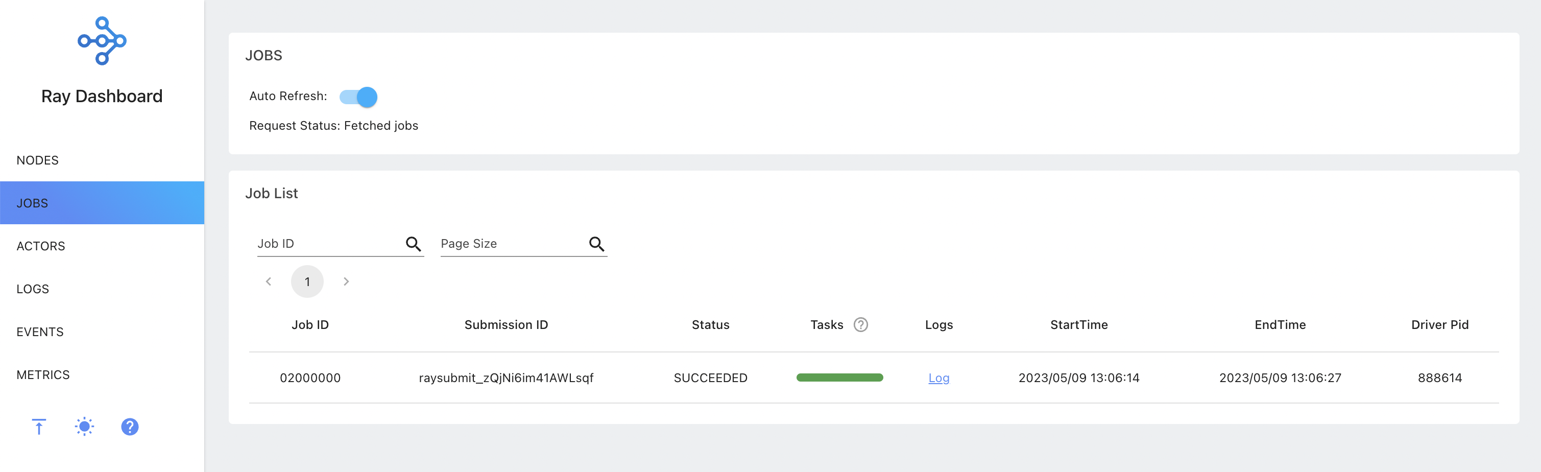
As suggested in the output of the submit command, you can see the logs and status of the job using its Submission_ID. You can also stop the job. The commands are

ray job logs {SUBMISSION_ID}
ray job status {SUBMISSION_ID}
ray job stop {SUBMISSION_ID}

Wow, that was a lot of stuff to cover! In this post, we've explored how to distribute computation jobs using Ray for faster and more efficient computation. Looking at an example of SGD, we’ve seen how we can significantly reduce the running time of our computations by at least a factor of 10 (this can vary depending on the computation resources you have and your tasks).

Before we go, I want to share some additional tips and insights I've gained through my experience with Ray. I'll also provide some visualizations of the SGD experiment that you might find interesting.

Additional tips

Port is not available

If you are getting this message

ConnectionError: Ray is trying to start at 192.168.1.2:6379, but is already running at 192.168.1.2:6379

when running ray start --head, this could be because the port is unavailable or another user is running a ray cluster. You can simply specify another port using

ray start --head --port {PORT_NUMBER}

PermissionError: [Errno 13]

You may also get

Permission denied: '/tmp/ray/ray_current_cluster'

when running the start command. This error is probably because another user is running a cluster, and Ray wants to use the same temp directory but does not have the write access. To fix this, you can create another temp directory and give the address using

ray start –head --temp-dir {PATH_TO_DIR}

File outputs

By default, if you use a relative path for your file outputs, Ray would write them in the tmp directory created for the run on each machine. If you want to save files, the best way is to mount shared cloud storage to both machines, but if you are not comfortable with that, you can just use absolute paths and collect the files from each machine.

Dashboard behind firewall

Sometimes server machines don’t expose all the ports to the outside world – where your computer may be. If you have ssh access, you can simply do a port forwarding using the -L option

ssh -L 8265:localhost:8265 user@server.domain.com

Now you can access the dashboard from your browser at localhost:8265

SGD Results

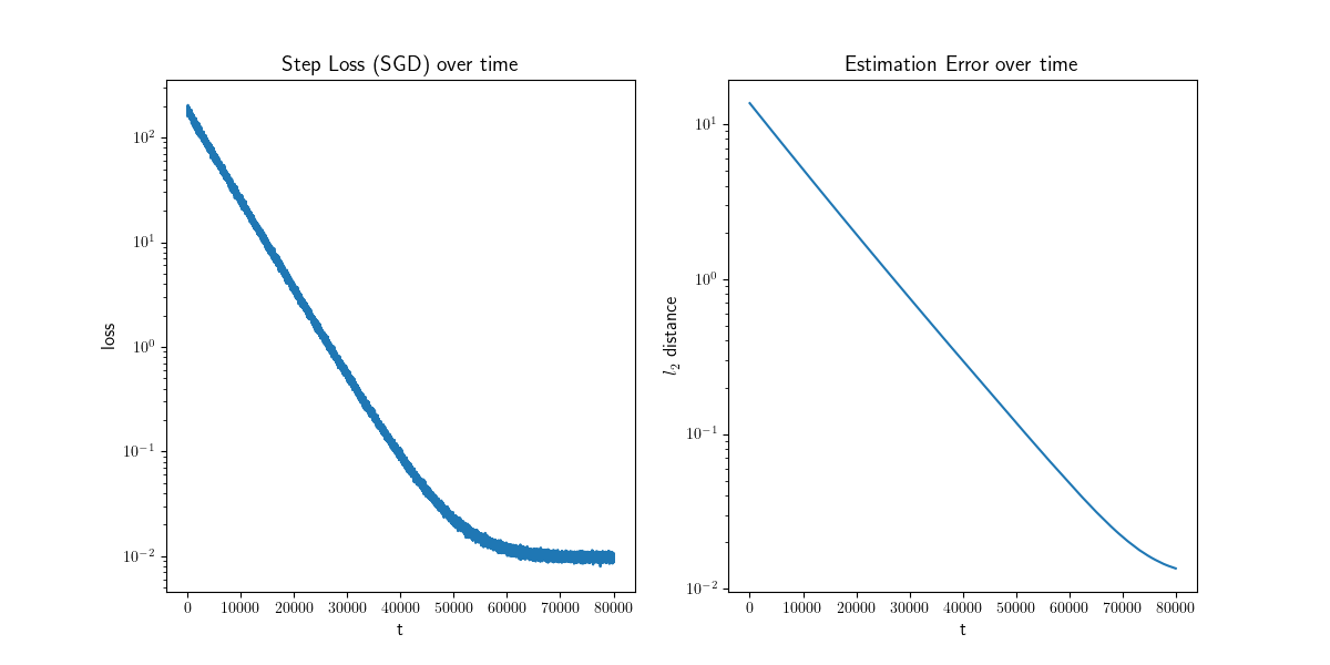
Finally, let's look at some of the results obtained from the SGD algorithm. The figure below provides insights into the learning procedure over time. On the left plot, we observe the squared loss at each step, representing the square of the distance between the true y value and the prediction. The right plot illustrates the \( l_2 \) distance between the estimated and true beta values. Notably, both plots exhibit a rapid initial decay, aligning with the expected \( O(1/t) + O(lr) \) convergence rates.

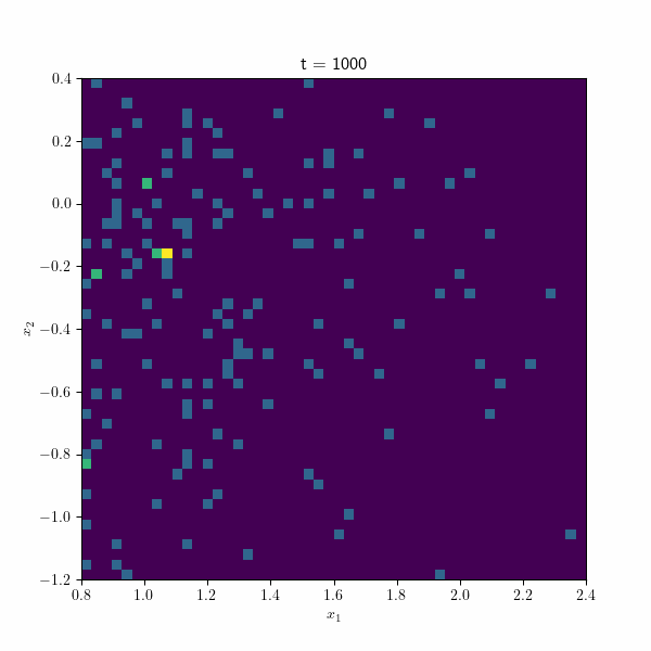
Moving on, the following figure showcases an animation presenting the histogram of the estimated betas along different repetitions of the algorithm through time. At each time step, the points collectively form a distribution resembling a normal distribution, gradually converging towards the true estimate by the end of the process. These visual representations provide valuable insights into the behavior and convergence of the SGD algorithm and demonstrate its effectiveness in approximating the true values.