You text a friend that you haven't seen for a long time. She/He replies, but not in a friendly manner, maybe just replying short answers like "I'm fine," "It's OK,"... After a week, you try again with the hope that you could schedule a phone/video call. She/He says it's a good idea and will inform you whenever she/he had time. Days pass, and nothing happens. I've recently been in these situations a few times, and maybe sometimes I was on the other side of the table. The question that comes up is how much you should continue this process, and when you should lose your hope. Or on the other side, how much should you expect your friends to give you time.

You may have been in these situations as well and may have solutions and techniques for yourself. When I was thinking about this problem weeks ago, I reminded two statistical inference approaches and tried to formalize the problem with that insight. Let's first take a look at the concepts.

Frequentist vs Bayesian

There are two main approaches in statistical inference, frequentist and bayesian. I will consider the parameter estimation task in this article and compare these two approaches in this task. The parameter estimation task rises in situations like estimating the average height of men in society or estimating the probability of getting heads when flipping a strange coin.

The frequentist approach only uses data and happenings of the past for its estimation. For instance, if the frequentist approach wants to estimate the probability of heads for a coin, it will use the previous results and counts the number of heads divided by the total number of trials. On the other hand, the Bayesian approach starts with an initial belief and updates it based on observations. To better explain these two, we will see the mathematics behind them for the coin flip problem.

Maths for coin flip problem

Frequentist's view

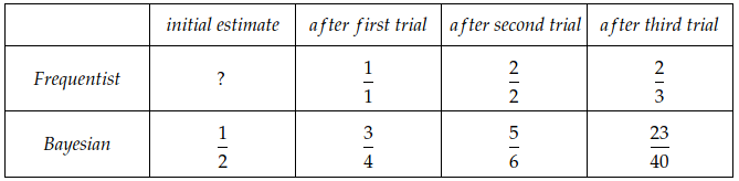
Consider we have a coin and have flipped it three times. The first two outcomes were heads, and the last one was tails. The frequentist approach starts without anything in mind because we don't have any prior experiences with the coin. After the first toss, as the outcome is heads, it estimates the probability to be \( \frac{1}{1} \). By the next two tosses, it will update the estimates to \( \frac{2}{2} \) and \( \frac{2}{3} \) consequently.

Bayesian's view

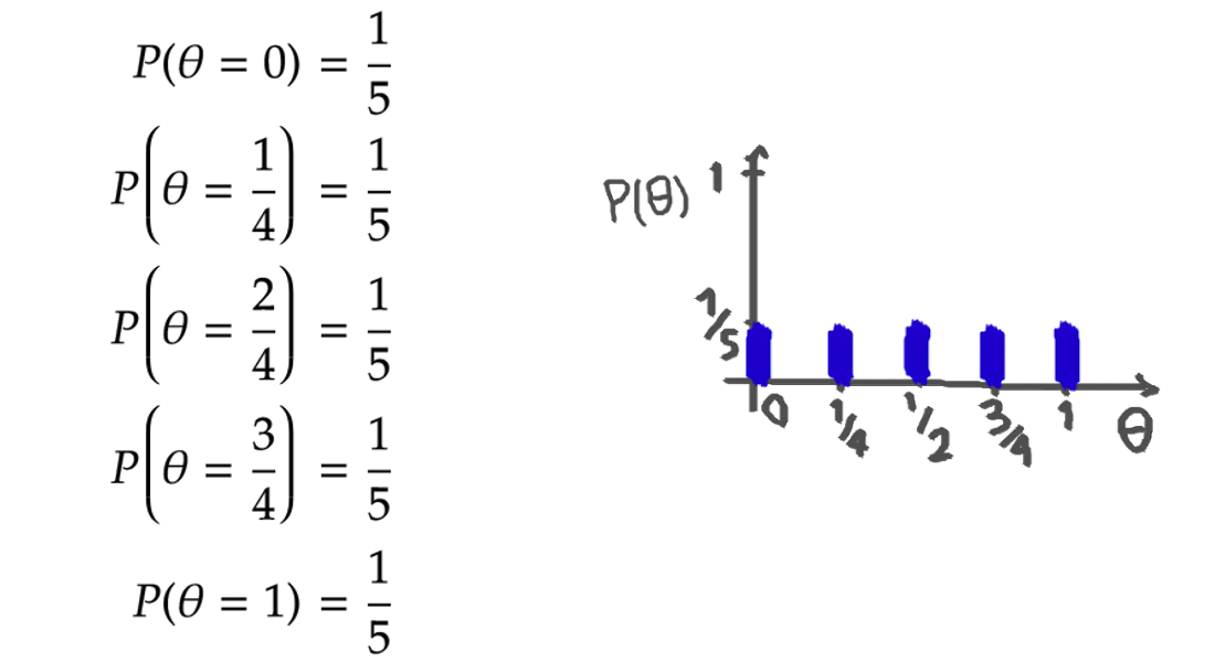
Analyzing the Bayesian approach is not that straightforward. First, we have to set the initial belief. For simplicity, I will consider the initial belief to have equal weights for these five potential values: \( \{0, \frac{1}{4}, \frac{2}{4}, \frac{3}{4}, 1\} \). We will consider the continuous initial belief in advance. The initial belief will be like:

The Bayesian approach uses the Bayes formula to update its beliefs after each observation. That is

In this example, \( \theta \) is any of the five potential probability values, and \( D \) is the observations. Let's compute the denominator for the first trial

This means before the first toss; we expect the outcome's probability of being heads to be \( \frac{1}{2} \). Now let's compute the new probabilities of parameters after the first toss.

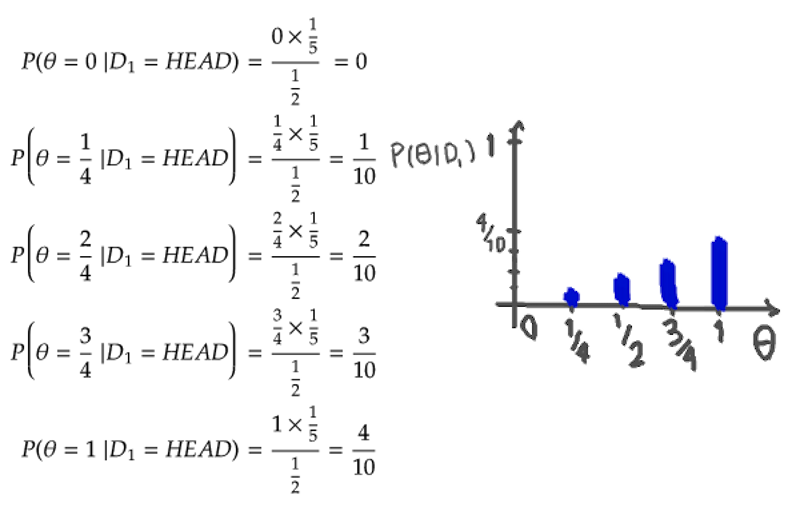
We see that after the first observation, the Bayesian approach stops putting any weight on the \( \theta = 0 \) condition, as it has seen one head so far. But unlike the frequentist approach, it doesn't immediately says that the probability of getting heads is one and still puts some weights on other possibilities. The calculation continues as

And finally

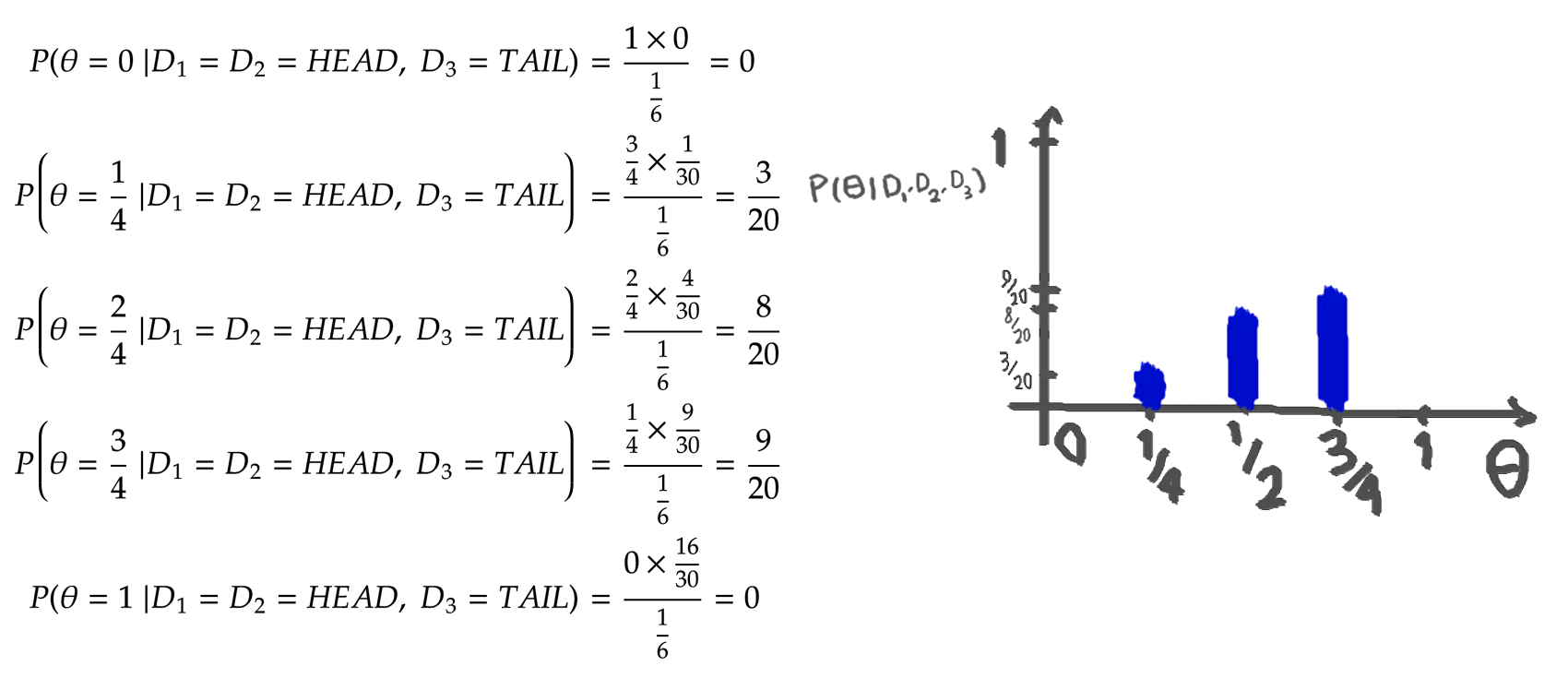
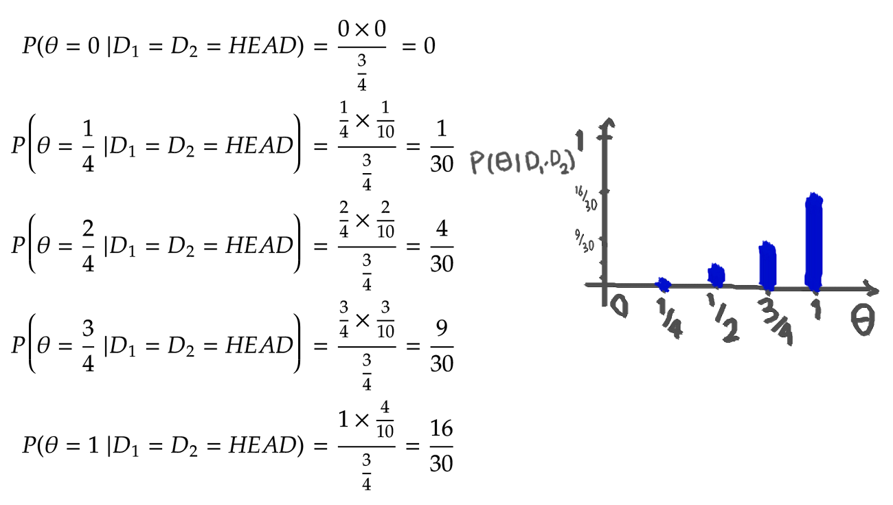
The Bayesian approach started with a uniform belief and updated it to give more weights on probabilities near one after seeing the first two heads. Following the third observation, it also removes the weight from \( \theta = 1 \) and skews the probabilities toward lower values.

Comparison

The frequentist approach gives a unique value for the estimated probability, while the Bayesian approach holds a probability distribution over the values. To reach one estimation value for the Bayesian method, we could take the expectation of the distribution. This way, the estimated probability of getting head in these two approaches will be:

Continuous version

While I had simplified the above example to a discrete version, you can play with the continuous version of the bayesian approach starting from uniform distribution in the section below.

I have taken the codes for this part from the Seeing Theory website. You can check it out and find other exciting visualizations for probability and statistics concepts.

In the continuous version, it is shown that the expectation of the Bayesian estimate is \( \frac{H + 1}{N + 2} \), where \( H \) is the number of heads and \( N \) is the total number of trials. On the other hand, the frequentist approach estimates the parameter to be \( \frac{H}{N} \). It is somehow like that the Bayesian method adds one head and one tail to the beginning of the sequence.

Back to the friendship case

The friendship scenarios are related to the coin flip example as I always have to estimate my friend's probability of responding appropriately. Then, maybe if I see the estimated probability is less than a threshold, I will lose my hope and don't text her/him the next time.

Let's define an optimistic line that indicates how hopeful you are about your friend's next behavior.

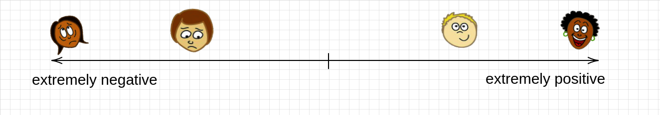
Notice: The faces are designed by Bonita90 from 99design

We want to see where each statistical approach will stand on this line in different situations.

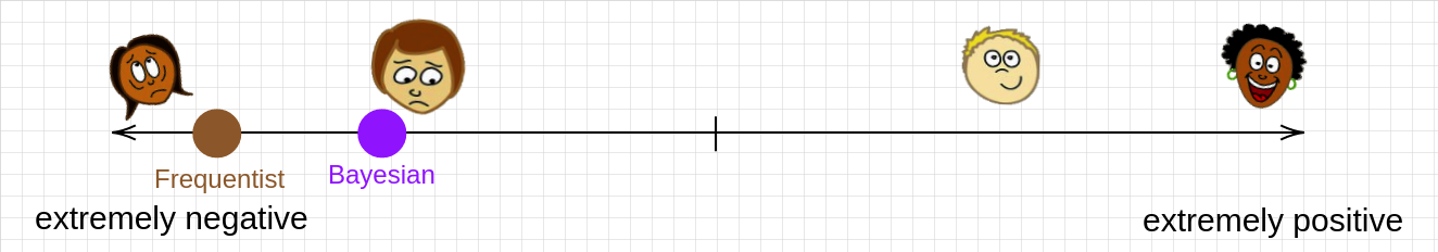
First, consider a situation where you had two unsuccessful attempts in connecting with your friend. The frequentist approach estimates the probability as \( \frac{0}{2} \) while the Bayesian approach's average estimate will be \( \frac{1}{4} \). So the line will be

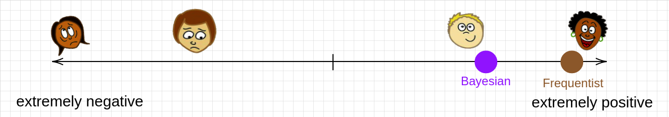
Oppositely, consider a situation where both of your first attempts were successful. Now the frequentist approach will estimate \( \frac{2}{2} \), and the Bayesian approach will estimate \( \frac{3}{4} \) on average. And we get

What about you? Where do you stand on the optimistic line in each of these scenarios? Of course, the answer may differ based on other factors, the details of what has happened between you, or maybe your personality and how much you like that friend. When I discussed this issue with some of my friends, some of them told me they are more optimistic in most cases because they know that everyone could face hard times and we have to be more patient in friendships.

While you are free to decide where you want to stand, personally, I think the frequentist approach is not a good option. I have some problems with this approach in both examples. It seems to me that the frequentist approach makes a harsh decision too early that may have harmful consequences. In the first example, it may lose hope early, causing a valuable friendship to die. On the other side, being optimistic based on a few good experiences may higher the expectations, and future bad outcomes may hurt you more. Overall, I think taking a moment before each decision and seeing it from this perspective is helpful. We could check how much evidence we have for our decisions and how confident we should be based on them.

Let me know your thoughts on this issue. Also, it will be great if you mention what other things we should consider in our modeling.

Thanks

Thank you, Matin Ansaripour, Bahar Salamatian, and Atia Hamidizadeh, for providing your time to discuss this topic, which helped me see the subject from new perspectives and organize this blog post. Additionally, Sina Rismanchian, Tannaz Azari, and again Bahar Salamatian to proofread the article and providing their opinions and excellent suggestions.